amplify automates routine pcr-based tasks - including plate planning, dilution making, visualizing, and analyzing.
Installation
You can install this package from GitHub with:
# install.packages("devtools")
devtools::install_github("KaiAragaki/amplify")Tidying qPCR data
Data exported from QuantStudio is fairly non-standard:
untidy_file_path <- system.file("extdata", "untidy-pcr-example.xls", package = "amplify")

untidy_file_path |>
  read_excel() |>
  select(1:10) |>
  head()
#> New names:
#> • `` -> `...3`
#> • `` -> `...4`
#> • `` -> `...5`
#> • `` -> `...6`
#> • `` -> `...7`
#> • `` -> `...8`
#> • `` -> `...9`
#> • `` -> `...10`
#> • `` -> `...11`
#> • `` -> `...12`
#> • `` -> `...13`
#> # A tibble: 6 × 10
#>   `Block Type`  `384-Well Block` ...3  ...4  ...5  ...6  ...7  ...8  ...9  ...10
#>   <chr>         <chr>            <chr> <chr> <chr> <chr> <chr> <chr> <chr> <chr>
#> 1 Calibration … Yes              <NA>  <NA>  <NA>  <NA>  <NA>  <NA>  <NA>  <NA>
#> 2 Calibration … 01-13-2020       <NA>  <NA>  <NA>  <NA>  <NA>  <NA>  <NA>  <NA>
#> 3 Calibration … Yes              <NA>  <NA>  <NA>  <NA>  <NA>  <NA>  <NA>  <NA>
#> 4 Calibration … 01-13-2020       <NA>  <NA>  <NA>  <NA>  <NA>  <NA>  <NA>  <NA>
#> 5 Calibration … Yes              <NA>  <NA>  <NA>  <NA>  <NA>  <NA>  <NA>  <NA>
#> 6 Calibration … 01-13-2020       <NA>  <NA>  <NA>  <NA>  <NA>  <NA>  <NA>  <NA>
amplify provides read_pcr to read in and tidy_lab (from {mop}) to automatically tidy these files. scrub (also from {mop}) can convert tidy_lab objects to data.frames
tidy_pcr <- untidy_file_path |>
  read_pcr() |>
  tidy_lab()
#>
#> ── Column specification ────────────────────────────────────────────────────────
#> cols(
#>   .default = col_double(),
#>   `Well Position` = col_character(),
#>   Omit = col_logical(),
#>   `Sample Name` = col_character(),
#>   `Target Name` = col_character(),
#>   Task = col_character(),
#>   Reporter = col_character(),
#>   Quencher = col_character(),
#>   Quantity = col_logical(),
#>   `Quantity Mean` = col_logical(),
#>   `Quantity SD` = col_logical(),
#>   CT = col_character(),
#>   `Delta Ct` = col_logical(),
#>   `Automatic Ct Threshold` = col_logical(),
#>   `Automatic Baseline` = col_logical(),
#>   Comments = col_logical()
#> )
#> ℹ Use `spec()` for the full column specifications.

tidy_pcr |>
  scrub() |>
  select(1:10) |>
  head()
#> # A tibble: 6 × 10
#>    .row  .col  well well_position omit  sample_name target_name task  reporter
#>   <dbl> <dbl> <dbl> <chr>         <lgl> <chr>       <chr>       <chr> <chr>
#> 1     1     1    NA <NA>          NA    <NA>        <NA>        <NA>  <NA>
#> 2     1     2    NA <NA>          NA    <NA>        <NA>        <NA>  <NA>
#> 3     1     3    NA <NA>          NA    <NA>        <NA>        <NA>  <NA>
#> 4     1     4    NA <NA>          NA    <NA>        <NA>        <NA>  <NA>
#> 5     1     5    NA <NA>          NA    <NA>        <NA>        <NA>  <NA>
#> 6     1     6    NA <NA>          NA    <NA>        <NA>        <NA>  <NA>
#> # ℹ 1 more variable: quencher <chr>
This works with both ddCt or standard curve result files.
Plotting qPCR results
Tidied results can be plotted using pcr_plot
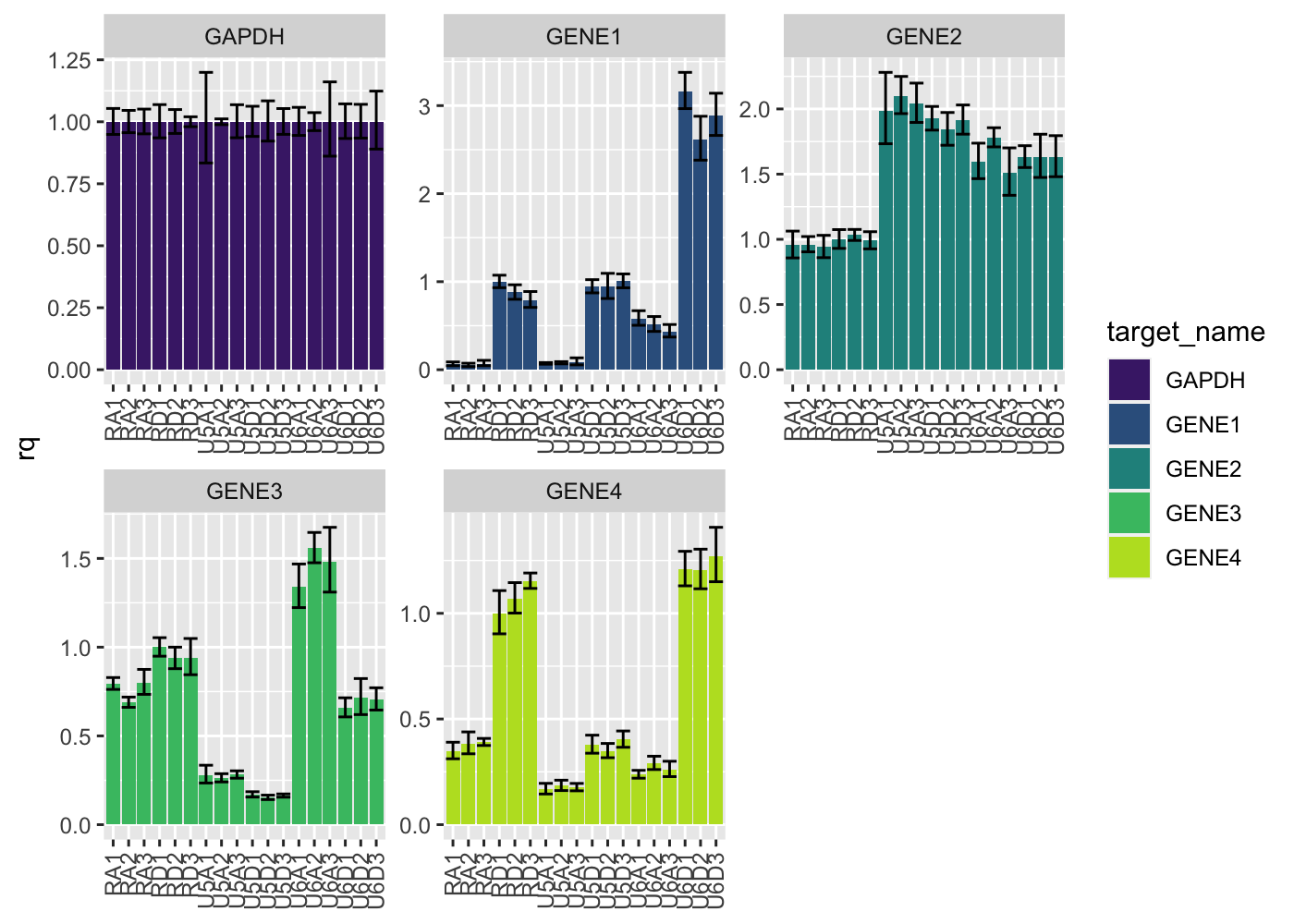
Additionally, overviews of plate features can be done using pcr_plate
tidy_pcr |>
  pcr_plate_view("target_name")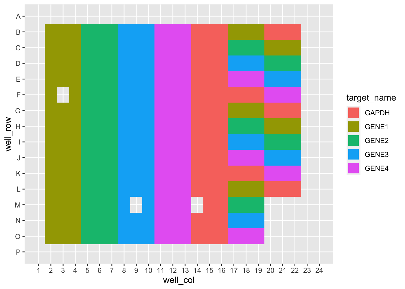
More details can be found in the Analyzing ddCt qPCR with amplify vignette.
Library Preparation Quantification
Library Preparation Quantification Calculation
RNA library preparation results output from Quantstudio can be tidied using pcr_tidy:
untidy_lib_path <- system.file("extdata", "untidy-standard-curve.xlsx", package = "amplify")
tidy_lib <- read_pcr(untidy_lib_path) |>
  tidy_lab(pad_zero = TRUE)
#>
#> ── Column specification ────────────────────────────────────────────────────────
#> cols(
#>   .default = col_double(),
#>   `Well Position` = col_character(),
#>   Omit = col_logical(),
#>   `Sample Name` = col_character(),
#>   `Target Name` = col_character(),
#>   Task = col_character(),
#>   Reporter = col_character(),
#>   Quencher = col_character(),
#>   CT = col_character(),
#>   `Automatic Ct Threshold` = col_logical(),
#>   `Automatic Baseline` = col_logical(),
#>   Comments = col_logical()
#> )
#> ℹ Use `spec()` for the full column specifications.
#> ! Multiple files in zip: reading ''[Content_Types].xml''
tidy_lib |>
  scrub() |>
  select(1:10) |>
  head()
#> # A tibble: 6 × 10
#>    .row  .col  well well_position omit  sample_name target_name task    reporter
#>   <dbl> <dbl> <dbl> <chr>         <lgl> <chr>       <chr>       <chr>   <chr>
#> 1     1     1     1 A1            FALSE Standard 01 Target 1    STANDA… FAM
#> 2     1     2     2 A2            FALSE Standard 01 Target 1    STANDA… FAM
#> 3     1     3     3 A3            FALSE Standard 01 Target 1    STANDA… FAM
#> 4     1     4    NA <NA>          NA    <NA>        <NA>        <NA>    <NA>
#> 5     1     5     5 A5            FALSE Sample 01   Target 1    UNKNOWN FAM
#> 6     1     6     6 A6            FALSE Sample 01   Target 1    UNKNOWN FAM
#> # ℹ 1 more variable: quencher <chr>
Calculating the concentration of library (before dilution) can be performed using pcr_lib_calc:
calc_lib <- pcr_lib_calc(tidy_lib)

calc_lib |>
  scrub() |>
  filter(task == "UNKNOWN") |>
  select(sample_name, concentration) |>
  head()
#> Adding missing grouping variables: `task`
#> # A tibble: 6 × 3
#> # Groups:   task [1]
#>   task    sample_name concentration
#>   <chr>   <chr>               <dbl>
#> 1 UNKNOWN Sample 06           2039.
#> 2 UNKNOWN Sample 06           2039.
#> 3 UNKNOWN Sample 06           2039.
#> 4 UNKNOWN Sample 12           1893.
#> 5 UNKNOWN Sample 12           1893.
#> 6 UNKNOWN Sample 12           1893.
Library preparation quantification quality control
We can generate useful plots to determine the quality of the quantification run by first using pcr_lib_qc:
qc <- calc_lib |>
  pcr_lib_qc()
lapply(qc, head, n = 3)
#> $standards
#> # A tibble: 3 × 19
#> # Groups:   sample_name [1]
#>   sample_name task     quantity_mean concentration quantity quant_actual   dil
#>   <chr>       <chr>            <dbl>         <dbl>    <dbl>        <dbl> <dbl>
#> 1 Standard 01 STANDARD            NA            NA     6.80         6.80     0
#> 2 Standard 01 STANDARD            NA            NA     6.80         6.80     0
#> 3 Standard 01 STANDARD            NA            NA     6.80         6.80     0
#> # ℹ 12 more variables: slope <dbl>, efficiency <dbl>, r_superscript_2 <dbl>,
#> #   ct <dbl>, no_po_mean <dbl>, no_po_sd <dbl>, keep <lgl>, keep_temp <lgl>,
#> #   mean_adj <dbl>, sd_adj <dbl>, quant_adj <dbl>, z <dbl>
#>
#> $samples
#> # A tibble: 3 × 19
#> # Groups:   sample_name [1]
#>   sample_name task    quantity_mean concentration quantity quant_actual   dil
#>   <chr>       <chr>           <dbl>         <dbl>    <dbl>        <dbl> <dbl>
#> 1 Sample 06   UNKNOWN          2.04         2039.     2.06         2.06    NA
#> 2 Sample 06   UNKNOWN          2.04         2039.     2.12         2.12    NA
#> 3 Sample 06   UNKNOWN          2.04         2039.     1.94         1.94    NA
#> # ℹ 12 more variables: slope <dbl>, efficiency <dbl>, r_superscript_2 <dbl>,
#> #   ct <dbl>, no_po_mean <dbl>, no_po_sd <dbl>, keep <lgl>, keep_temp <lgl>,
#> #   mean_adj <dbl>, sd_adj <dbl>, quant_adj <dbl>, z <dbl>
#>
#> $sample_summary
#> # A tibble: 3 × 3
#>   sample_name quantity_mean quant_adj
#>   <chr>               <dbl>     <dbl>
#> 1 Sample 01           0.599     0.599
#> 2 Sample 02           1.05      1.05
#> 3 Sample 03           1.37      1.39
#>
#> $standard_summary
#> # A tibble: 3 × 4
#>   sample_name   dil quantity_mean quant_actual
#>   <chr>       <dbl>         <dbl>        <dbl>
#> 1 Standard 01  0           6.80         6.80
#> 2 Standard 02  9.27        0.680        0.734
#> 3 Standard 03 12.2         0.0680       0.0603
#>
#> $outliers
#> # A tibble: 3 × 19
#> # Groups:   sample_name [1]
#>   sample_name task     quantity_mean concentration quantity quant_actual   dil
#>   <chr>       <chr>            <dbl>         <dbl>    <dbl>        <dbl> <dbl>
#> 1 Standard 01 STANDARD            NA            NA     6.80         6.80     0
#> 2 Standard 01 STANDARD            NA            NA     6.80         6.80     0
#> 3 Standard 01 STANDARD            NA            NA     6.80         6.80     0
#> # ℹ 12 more variables: slope <dbl>, efficiency <dbl>, r_superscript_2 <dbl>,
#> #   ct <dbl>, no_po_mean <dbl>, no_po_sd <dbl>, keep <lgl>, keep_temp <lgl>,
#> #   mean_adj <dbl>, sd_adj <dbl>, quant_adj <dbl>, z <dbl>
These data, by themselves, are not particularly useful. However, a suite of QC plotting functions can be used upon these data to give insight, such as:
qc |> pcr_lib_qc_plot_conc()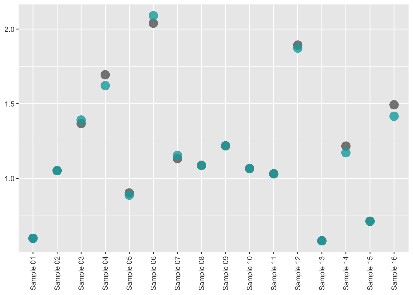
All QC plotting functions can be run and generate a report using pcr_lib_qc_report.
qc |> pcr_lib_qc_report("path/to/my/report.html")More information about the plots available, as well as their interpretations, can be found in Performing Library Quantification QC