Introduction
Let’s consider a relatively full-featured, practical use case for
reclanc. In this vignette, we’ll go over the basics of
fitting models, as well as how to leverage tidymodels to do
more elaborate things like resampling and tuning hyperparameters. We’ll
fit a final model, then use that to predict subtypes of an entirely new
dataset.
This vignette tries to assume very little knowledge about machine
learning or tidymodels.
Fitting
A simple fit
Let’s start with the fitting procedure. We first need gene expression data.
The data I’m using is from Sjödahl et al. (2012). It contains RNA expression from 308 bladder cancer tumors.
lund <- s3readRDS("lund.rds", "reclanc-lund", region = "us-east-2")
lund
#> ExpressionSet (storageMode: lockedEnvironment)
#> assayData: 16940 features, 308 samples
#>   element names: exprs
#> protocolData: none
#> phenoData
#>   sampleNames: UC_0001_1 UC_0002_1 ... UC_0785_1 (308 total)
#>   varLabels: title source ... sample (16 total)
#>   varMetadata: labelDescription
#> featureData: none
#> experimentData: use 'experimentData(object)'
#> Annotation:
In their paper, Sjödahl et al. used the transcriptional data to classify the tumors into seven molecular subtypes (MS):
table(lund$molecular_subtype)
#>
#>    MS1a    MS1b  MS2a.1  MS2a.2  MS2b.1 MS2b2.1 MS2b2.2
#>      53      78      30      55      43      20      29
We’d like to apply this subtype framework to other datasets. To do this, we first need to generate centroids. Before we can begin, though, we need to convert our outcomes to factors. In this case, our outcomes are the molecular subtypes:
lund$molecular_subtype <- factor(lund$molecular_subtype)In its simplest form, since clanc accepts
ExpressionSet objects, we could do the following and be
done with it:
simple_centroids <- clanc(lund, classes = "molecular_subtype", active = 5)
head(simple_centroids$centroids)
#>   class    gene expression pooled_sd active     prior
#> 1  MS1a   CXCL1   6.534490 0.8749133      5 0.1428571
#> 2  MS1a     MMD   7.922508 0.6429620      5 0.1428571
#> 3  MS1a C9orf19   8.378910 0.7510552      5 0.1428571
#> 4  MS1a    BNC1   5.297095 0.2106762      5 0.1428571
#> 5  MS1a  SLFN11   7.362887 0.6824663      5 0.1428571
#> 6  MS1a    CRAT   6.004517 0.3425669      5 0.1428571
The problem with this method, though, is we have no idea if this is a
good fit or not. active is an argument that specifies the
number of genes that are used as distinguishing features for a given
class. In this case, each class will find 5 genes that have expression
patterns peculiar to that given molecular subtype, and each subtype will
have 7 (the total number of subtypes) x 5 (number of active genes) = 35
genes in it (see my blog post or -
better yet - the
original paper for more details). Could we have gotten a better fit
with more genes? Are we selecting more genes than we need? How would we
know?
Setting the stage for more elaborate analyses
Before we can get started on tackling these larger questions, let’s
take a brief detour to the land of tidymodels.
tidymodels is a collection of packages that make running
and tuning algorithms like this much less painful and much more
standardized.
In order to leverage tidymodels, we need to buy-in to
their data structures.
(Aside: I don’t mean to make the buy-in sound begrudging. When I say
need, I really mean it: we’re going to be specifying very long formulas,
which for some reason R really, really hates. Emil Hvitfeldt
recently (at time of writing) has allowed
tidymodels to handle long formulas gracefully, so using
tidymodels infrastructure is a gift, not a chore.)
Many tidymodels workflows begin with a model
specification. The rationale behind this is to separate the
model specification step from the model fitting step
(whereas in base R, they generally all happen at once).
reclanc makes it easy to specify a model by adding a custom
engine to parsnip::discrim_linear, so specifying a model
looks like this:
mod <- discrim_linear() |>
  set_engine(
    engine = "clanc", # Note: "clanc", not "reclanc"
    active = 5
  )
This mod doesn’t do anything - and that’s kind of the
point: it only specifies the model we will later fit with, but doesn’t
do any fitting itself. This allows us to reuse the specification across
our code.
The next step is to wrangle our data a bit to be in a ‘wide’ format, where all columns are outcomes (classes) and predictors (genes), and all rows are observations (samples):
wrangled <- data.frame(class = lund$molecular_subtype, t(exprs(lund)))
head(wrangled[1:5])
#>            class LOC23117   FCGR2B    TRIM44 C15orf39
#> UC_0001_1   MS1b 5.565262 5.306654  9.305053 6.430063
#> UC_0002_1 MS2b.1 5.505854 5.731128  9.242790 7.265748
#> UC_0003_1 MS2a.2 5.336140 5.540470  9.888668 7.244976
#> UC_0006_2 MS2b.1 5.576748 5.847743  9.408895 7.377358
#> UC_0007_1 MS2a.2 5.414919 5.510507 10.482469 6.435552
#> UC_0008_1 MS2b.1 5.279174 5.633093  9.112754 7.057977
Finally, we specify a formula for fitting the model. This uses the
recipes package from tidymodels. While this is
a delightful package that can help you preprocess your data, it’s out of
the scope of this vignette. Instead, just think of it as a way to
specify a formula that keeps R from blowing up:
# Note that the recipe requires 'template data'
recipe <- recipe(class ~ ., wrangled)
We can bundle our model specification (mod) and our
preprocessing steps (recipe, which is just a formula) into
a workflow:
wf <- workflow() |>
  add_recipe(recipe) |>
  add_model(mod)
wf
#> ══ Workflow ════════════════════════════════════════════════════════════════════
#> Preprocessor: Recipe
#> Model: discrim_linear()
#>
#> ── Preprocessor ────────────────────────────────────────────────────────────────
#> 0 Recipe Steps
#>
#> ── Model ───────────────────────────────────────────────────────────────────────
#> Linear Discriminant Model Specification (classification)
#>
#> Engine-Specific Arguments:
#>   active = 5
#>
#> Computational engine: clanc
Now we can fit our model:
tidymodels_fit <- fit(wf, data = wrangled)
head(extract_fit_parsnip(tidymodels_fit)$fit$centroids)
#>   class    gene expression pooled_sd active     prior
#> 1  MS1a   CXCL1   6.534490 0.8749133      5 0.1428571
#> 2  MS1a     MMD   7.922508 0.6429620      5 0.1428571
#> 3  MS1a C9orf19   8.378910 0.7510552      5 0.1428571
#> 4  MS1a    BNC1   5.297095 0.2106762      5 0.1428571
#> 5  MS1a  SLFN11   7.362887 0.6824663      5 0.1428571
#> 6  MS1a    CRAT   6.004517 0.3425669      5 0.1428571
You’ll notice that our results are the same as what we saw
previously, demonstrating that while we’re using tidymodels
rather than base R, we’re still doing the same thing.
Measuring fit accuracy with cross-validation
Now that we’ve dialed in to the tidymodels framework, we
can do a lot of elaborate things with ease. One of our concerns is
whether 5 active genes was a good choice (active = 5). A
somewhat simple way to determine how good our choice of 5 genes is to
use cross-validation.
Cross-validation allows us to test how good our fit is by training our
model on, say, 80% of our data, and testing it on the rest (see the
Wikipedia diagram of a k-fold cross validation). This allows us to get a
measure of how good our fit is, without having to break out our actual
test data - which in general should only be used when we’re ready to
finalize our model.
Speaking of test data, let’s go ahead and split that off now. We’ll lock our test data away and only use it once we’ve fit our final model. Until then, we’ll use cross validation to assess how good the fit is, essentially using our training data as its own testing data.
Of course, tidymodels makes this easy too, by using
rsample::initial_split:
set.seed(123)
splits <- initial_split(wrangled, prop = 0.8, strata = class)
train <- training(splits)
test <- testing(splits)
train and test are just subsets of the
original data, containing 80% and 20% of the original data
(respectively). It also tries to maintain the relative proportions of
each of the classes within each of the datasets (because we set
strata = class):
round(prop.table(table(train$class)), 2)
#>
#>    MS1a    MS1b  MS2a.1  MS2a.2  MS2b.1 MS2b2.1 MS2b2.2
#>    0.17    0.25    0.10    0.18    0.15    0.07    0.08
round(prop.table(table(test$class)), 2)
#>
#>    MS1a    MS1b  MS2a.1  MS2a.2  MS2b.1 MS2b2.1 MS2b2.2
#>    0.19    0.27    0.08    0.16    0.11    0.05    0.16
Creating folds for cross validation is nearly the same as
initial_split:
folds <- vfold_cv(train, v = 5, strata = class)
folds
#> #  5-fold cross-validation using stratification
#> # A tibble: 5 × 2
#>   splits           id
#>   <list>           <chr>
#> 1 <split [193/51]> Fold1
#> 2 <split [193/51]> Fold2
#> 3 <split [195/49]> Fold3
#> 4 <split [197/47]> Fold4
#> 5 <split [198/46]> Fold5
We can reuse our workflow wf, which contains our model
and formula. The only difference is that we use
fit_resamples, and we specify a metric we want to use to
measure how good our fit is (remember that every fold has a chunk of
data it uses to test the fit). For simplicity, let’s use accuracy:
fits <- fit_resamples(
  wf,
  folds,
  metrics = metric_set(accuracy)
)
#> 35/35 (100%) genes in centroids found in data
#> 35/35 (100%) genes in centroids found in data
#> 35/35 (100%) genes in centroids found in data
#> 35/35 (100%) genes in centroids found in data
#> 35/35 (100%) genes in centroids found in data
fits
#> # Resampling results
#> # 5-fold cross-validation using stratification
#> # A tibble: 5 × 4
#>   splits           id    .metrics         .notes
#>   <list>           <chr> <list>           <list>
#> 1 <split [193/51]> Fold1 <tibble [1 × 4]> <tibble [0 × 3]>
#> 2 <split [193/51]> Fold2 <tibble [1 × 4]> <tibble [0 × 3]>
#> 3 <split [195/49]> Fold3 <tibble [1 × 4]> <tibble [0 × 3]>
#> 4 <split [197/47]> Fold4 <tibble [1 × 4]> <tibble [0 × 3]>
#> 5 <split [198/46]> Fold5 <tibble [1 × 4]> <tibble [0 × 3]>
We can then extract our accuracy metrics by using
collect_metrics, which roots around in each of our fits and
helpfully extracts the metrics, aggregates them, and calculated the
standard error:
metrics <- collect_metrics(fits)
metrics
#> # A tibble: 1 × 6
#>   .metric  .estimator  mean     n std_err .config
#>   <chr>    <chr>      <dbl> <int>   <dbl> <chr>
#> 1 accuracy multiclass 0.737     5  0.0289 Preprocessor1_Model1
Our model has an accuracy of about 74%. Applying this model to our testing data:
# Fit a model using *all* of our training data
final_fit <- clanc(class ~ ., train, active = 5)

# Use it to predict the (known) classes of our test data
preds <- predict(final_fit, new_data = test, type = "class")
#> 35/35 (100%) genes in centroids found in data
w_preds <- cbind(preds, test)
# Compare known class vs predicted class
metric <- accuracy(w_preds, class, .pred_class)
metric
#> # A tibble: 1 × 3
#>   .metric  .estimator .estimate
#>   <chr>    <chr>          <dbl>
#> 1 accuracy multiclass     0.734
Note that our testing data accuracy (%) approximates the training data accuracy (74%).
Tuning hyperparameters with tune
Now we at least have some measure of how good our model
fits, but could it be better with more genes? Could we get away with
fewer? Running the same command over and over again with different
numbers is a drag - fortunately, there’s yet another beautiful package
to help us: tune.
To use tune, we need to re-specify our model to let
tune know what parameters we want to tune:
tune_mod <- discrim_linear() |>
  set_engine(
    engine = "clanc",
    active = tune()
  )
We could update our previous workflow using
update_model, but let’s just declare a new one:
tune_wf <- workflow() |>
  add_recipe(recipe) |>
  add_model(tune_mod)
We then have to specify a range of values of active to
try:
values <- data.frame(active = seq(from = 1, to = 50, by = 4))
values
#>    active
#> 1       1
#> 2       5
#> 3       9
#> 4      13
#> 5      17
#> 6      21
#> 7      25
#> 8      29
#> 9      33
#> 10     37
#> 11     41
#> 12     45
#> 13     49
We can then fit our folds using the spread of values we
chose:
# This is going to take some time, since we're fitting 5 folds 13 times each.
tuned <- tune_grid(
  tune_wf,
  folds,
  metrics = metric_set(accuracy),
  grid = values
)
tuned
#> # Tuning results
#> # 5-fold cross-validation using stratification
#> # A tibble: 5 × 4
#>   splits           id    .metrics          .notes
#>   <list>           <chr> <list>            <list>
#> 1 <split [193/51]> Fold1 <tibble [13 × 5]> <tibble [0 × 3]>
#> 2 <split [193/51]> Fold2 <tibble [13 × 5]> <tibble [0 × 3]>
#> 3 <split [195/49]> Fold3 <tibble [13 × 5]> <tibble [0 × 3]>
#> 4 <split [197/47]> Fold4 <tibble [13 × 5]> <tibble [0 × 3]>
#> 5 <split [198/46]> Fold5 <tibble [13 × 5]> <tibble [0 × 3]>
As before, we can collect our metrics - this time, however, we have a
summary of metrics for each of values for active:
tuned_metrics <- collect_metrics(tuned)
tuned_metrics
#> # A tibble: 13 × 7
#>    active .metric  .estimator  mean     n std_err .config
#>     <dbl> <chr>    <chr>      <dbl> <int>   <dbl> <chr>
#>  1      1 accuracy multiclass 0.585     5  0.0368 Preprocessor1_Model01
#>  2      5 accuracy multiclass 0.737     5  0.0289 Preprocessor1_Model02
#>  3      9 accuracy multiclass 0.748     5  0.0496 Preprocessor1_Model03
#>  4     13 accuracy multiclass 0.781     5  0.0403 Preprocessor1_Model04
#>  5     17 accuracy multiclass 0.770     5  0.0280 Preprocessor1_Model05
#>  6     21 accuracy multiclass 0.774     5  0.0335 Preprocessor1_Model06
#>  7     25 accuracy multiclass 0.785     5  0.0378 Preprocessor1_Model07
#>  8     29 accuracy multiclass 0.794     5  0.0319 Preprocessor1_Model08
#>  9     33 accuracy multiclass 0.773     5  0.0281 Preprocessor1_Model09
#> 10     37 accuracy multiclass 0.790     5  0.0295 Preprocessor1_Model10
#> 11     41 accuracy multiclass 0.794     5  0.0339 Preprocessor1_Model11
#> 12     45 accuracy multiclass 0.815     5  0.0267 Preprocessor1_Model12
#> 13     49 accuracy multiclass 0.815     5  0.0277 Preprocessor1_Model13
Or graphically:
ggplot(tuned_metrics, aes(active, mean)) +
  geom_line() +
  coord_cartesian(ylim = c(0, 1)) +
  labs(x = "Number Active Genes", y = "Accuracy")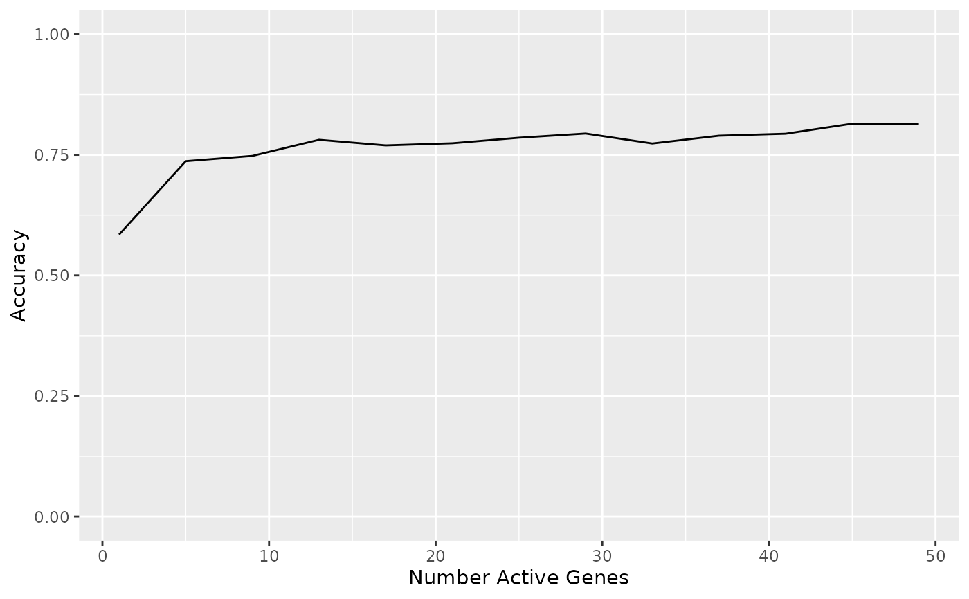
It looks like we read maximal accuracy at around 21 genes - let’s choose 20 genes for a nice round number:
final_fit_tuned <- clanc(class ~ ., data = train, active = 20)
# Use it to predict the (known) classes of our test data:
preds <- predict(final_fit_tuned, new_data = test, type = "class")
#> 140/140 (100%) genes in centroids found in data
w_preds <- cbind(preds, test)
# Compare known class vs predicted class:
metric <- accuracy(w_preds, class, .pred_class)
metric
#> # A tibble: 1 × 3
#>   .metric  .estimator .estimate
#>   <chr>    <chr>          <dbl>
#> 1 accuracy multiclass     0.812
It looks like our accuracy is a little better now that we’ve chosen an optimal number of active genes.
Predicting
Now we want to apply our classifier to new data. Our second dataset is RNAseq data from 30 bladder cancer cell lines:
library(cellebrate)
cell_rna
#> class: DESeqDataSet
#> dim: 18548 30
#> metadata(1): version
#> assays(2): counts rlog_norm_counts
#> rownames(18548): TSPAN6 TNMD ... MT-ND5 MT-ND6
#> rowData names(0):
#> colnames(30): 1A6 253JP ... UC7 UC9
#> colData names(5): cell bsl lum call clade
Predicting is incredibly simple. Since we’re using a different
sequencing method (RNAseq vs array-based sequencing), it probably makes
sense to use a correlation based classification rather than the original
distance-based metric used in the original ClaNC package. We can do that
by specifying type = "numeric" and then whatever
correlation method we prefer.
cell_preds <- predict(
  final_fit_tuned,
  cell_rna,
  assay = 2,
  type = "numeric",
  method = "spearman"
)
#> 118/140 (84%) genes in centroids found in data

out <- cbind(colData(cell_rna), cell_preds) |>
  as_tibble()

out
#> # A tibble: 30 × 12
#>    cell     bsl    lum call  clade            .pred_MS1a .pred_MS1b .pred_MS2a.1
#>    <chr>  <dbl>  <dbl> <chr> <fct>                 <dbl>      <dbl>        <dbl>
#>  1 1A6     99.0   1.02 BSL   Epithelial Other     0.0600      0.224        0.149
#>  2 253JP   76.6  23.4  BSL   Unknown              0.0574      0.240        0.219
#>  3 5637    98.5   1.46 BSL   Epithelial Other     0.0958      0.243        0.160
#>  4 BV      49.9  50.1  LUM   Unknown              0.0758      0.262        0.238
#>  5 HT1197  56.0  44.0  BSL   Epithelial Other     0.119       0.288        0.224
#>  6 HT1376  10.9  89.1  LUM   Epithelial Other     0.100       0.277        0.238
#>  7 J82     98.1   1.91 BSL   Mesenchymal          0.127       0.292        0.219
#>  8 RT112    0   100    LUM   Luminal Papilla…     0.173       0.380        0.294
#>  9 RT4      0   100    LUM   Luminal Papilla…     0.134       0.317        0.257
#> 10 RT4V6    0   100    LUM   Luminal Papilla…     0.143       0.207        0.165
#> # ℹ 20 more rows
#> # ℹ 4 more variables: .pred_MS2a.2 <dbl>, .pred_MS2b.1 <dbl>,
#> #   .pred_MS2b2.1 <dbl>, .pred_MS2b2.2 <dbl>
plotting_data <- out |>
  pivot_longer(cols = starts_with(".pred"))

plotting_data |>
  ggplot(aes(cell, value, color = name)) +
  geom_point() +
  facet_grid(~clade, scales = "free_x", space = "free_x")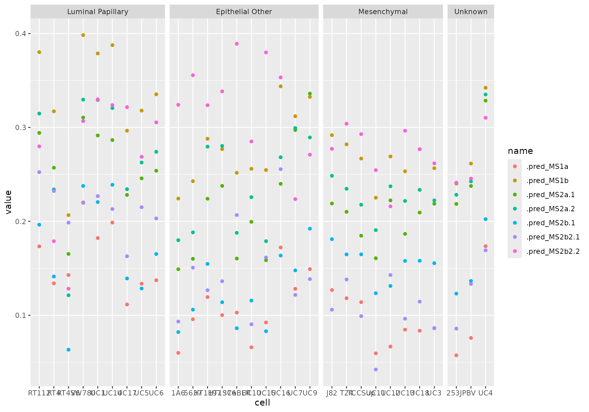
In the Sjödahl paper, the seven subtypes were simplified into five subtypes by merging some of the two that had similar biological pathways activated. To ease interpretation, we can do that too:
table <- plotting_data |>
  summarize(winner = name[which.max(value)], .by = c(cell, clade)) |>
  mutate(
    five = case_when(
      winner %in% c(".pred_MS1a", ".pred_MS1b") ~ "Urobasal A",
      winner %in% c(".pred_MS2a.1", ".pred_MS2a.2") ~ "Genomically unstable",
      winner == ".pred_MS2b.1" ~ "Infiltrated",
      winner == ".pred_MS2b2.1" ~ "Uro-B",
      winner == ".pred_MS2b2.2" ~ "SCC-like"
    )
  ) |>
  relocate(cell, five, clade)

print(table, n = 30)
#> # A tibble: 30 × 4
#>    cell   five                 clade             winner
#>    <chr>  <chr>                <fct>             <chr>
#>  1 1A6    SCC-like             Epithelial Other  .pred_MS2b2.2
#>  2 253JP  SCC-like             Unknown           .pred_MS2b2.2
#>  3 5637   SCC-like             Epithelial Other  .pred_MS2b2.2
#>  4 BV     Urobasal A           Unknown           .pred_MS1b
#>  5 HT1197 SCC-like             Epithelial Other  .pred_MS2b2.2
#>  6 HT1376 SCC-like             Epithelial Other  .pred_MS2b2.2
#>  7 J82    Urobasal A           Mesenchymal       .pred_MS1b
#>  8 RT112  Urobasal A           Luminal Papillary .pred_MS1b
#>  9 RT4    Urobasal A           Luminal Papillary .pred_MS1b
#> 10 RT4V6  Urobasal A           Luminal Papillary .pred_MS1b
#> 11 SCaBER SCC-like             Epithelial Other  .pred_MS2b2.2
#> 12 SW780  Urobasal A           Luminal Papillary .pred_MS1b
#> 13 T24    SCC-like             Mesenchymal       .pred_MS2b2.2
#> 14 TCCSup SCC-like             Mesenchymal       .pred_MS2b2.2
#> 15 UC10   SCC-like             Epithelial Other  .pred_MS2b2.2
#> 16 UC11   SCC-like             Mesenchymal       .pred_MS2b2.2
#> 17 UC12   Urobasal A           Mesenchymal       .pred_MS1b
#> 18 UC13   SCC-like             Mesenchymal       .pred_MS2b2.2
#> 19 UC14   Urobasal A           Luminal Papillary .pred_MS1b
#> 20 UC15   SCC-like             Epithelial Other  .pred_MS2b2.2
#> 21 UC16   SCC-like             Epithelial Other  .pred_MS2b2.2
#> 22 UC17   SCC-like             Luminal Papillary .pred_MS2b2.2
#> 23 UC18   SCC-like             Mesenchymal       .pred_MS2b2.2
#> 24 UC1    Urobasal A           Luminal Papillary .pred_MS1b
#> 25 UC3    SCC-like             Mesenchymal       .pred_MS2b2.2
#> 26 UC4    Urobasal A           Unknown           .pred_MS1b
#> 27 UC5    Urobasal A           Luminal Papillary .pred_MS1b
#> 28 UC6    Urobasal A           Luminal Papillary .pred_MS1b
#> 29 UC7    Urobasal A           Epithelial Other  .pred_MS1b
#> 30 UC9    Genomically unstable Epithelial Other  .pred_MS2a.1