usage

library(blotbench)

Introduction

When preparing western blots for presentation, typical workflows at one point usually involve cropping the blots in something like PhotoShop, GIMP, FIJI, etc. Because this manipulation was done in a separate program, usually the best we can do in terms of reproducibility is by providing the original, unmodified images along with the cropped version.

This is fine - it certainly is convenient and I don’t blame anyone for doing it (particularly busy scientists). There are methods for declaratively doing image manipulations in R (particularly magick and EBImage), but they aren’t nearly as convenient as the real-time visual feedback of typical photo-editing software - the guess-then-render-repeat loop of trying to find the perfect cropping geometry for an image without this visual feedback is tedious at best, and a hard-sell if you’re trying to get others to join the reproducibility movement.

blotbench attempts to solve this by providing a Shiny app within the package to perform rudimentary image manipulations with visual feedback. This app outputs code that should be written to create these transformations (rather than the image itself) so the declarative and reproducible benefits of a script can be reaped while still leveraging the convenience of a graphical interface.

In addition, blotbench introduces a new object (a wb object) that can store row and column annotation much like a SummarizedExperiment. This provides additional benefits such as intuitive indexing (to allow you to treat a blot image almost like a data.frame) and automatic annotation.

Creating a `wb` object

A wb object is composed of 4 components:

imgs: A vector of image-magick images
col_annot: A data.frame containing lane annotation, one line for each column, with the top row referring to the left-most lane
row_annot: A data.frame containing names of the protein blotted for in each image.
transforms: A data.frame containing information detailing what transformations should be performed on the image for presentation.

When creating a wb object, you typically will not specify the transforms at the outset, and both col_annot and row_annot are optional. At bare minimum, you need to supply a vector of image-magick images. To show you the full power of blotbench though, I’m going to supply arguments 1-3.

First, let’s introduce our images.

Our experiment was a timecourse of cells exposed to a drug (erdafitinib - an FGFR inhibitor). We blotted for three proteins - TRAIL, PARP, and Actin.

Here is our PARP blot:

library(magick)
#> Linking to ImageMagick 6.9.11.60
#> Enabled features: fontconfig, freetype, fftw, heic, lcms, pango, webp, x11
#> Disabled features: cairo, ghostscript, raw, rsvg
#> Using 4 threads
parp <- image_read(system.file("extdata", "parp.tif", package = "blotbench"))
plot(parp)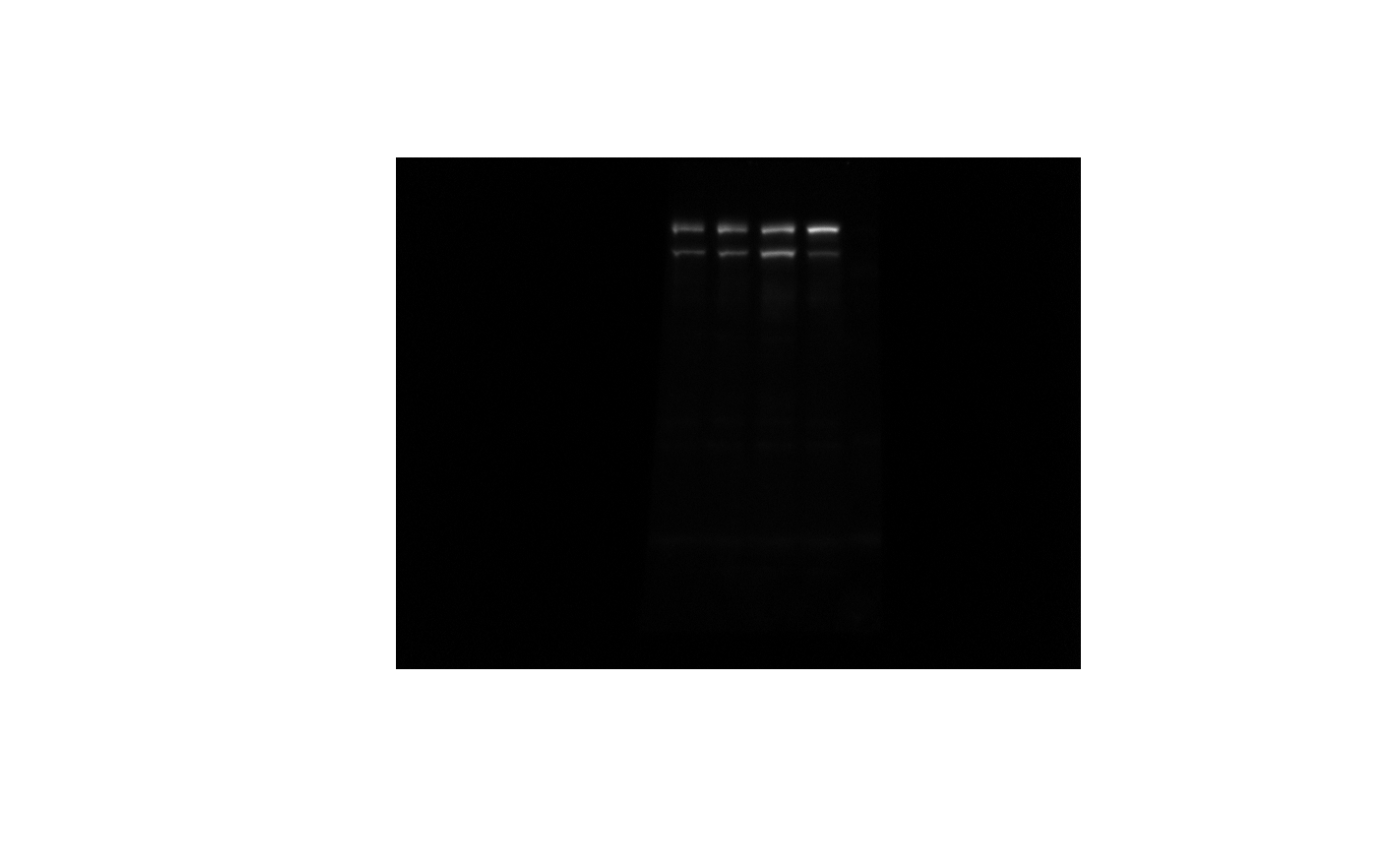

After blotting for PARP, we probed the same blot again for TRAIL:

trail <- image_read(system.file("extdata", "trail.tif", package = "blotbench"))
plot(trail)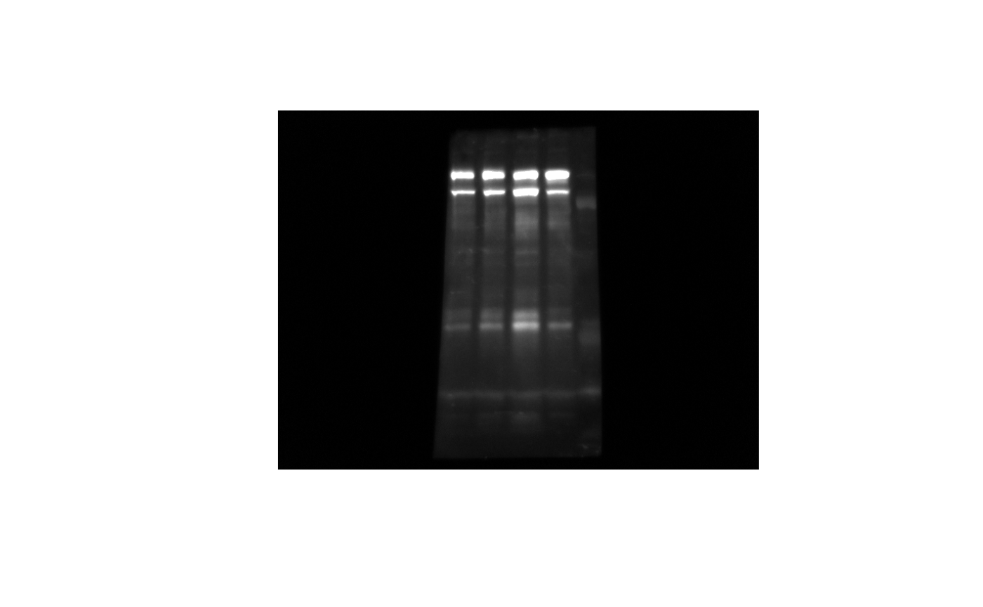

And finally for Actin:

actin <- image_read(system.file("extdata", "actin.tif", package = "blotbench"))
plot(actin)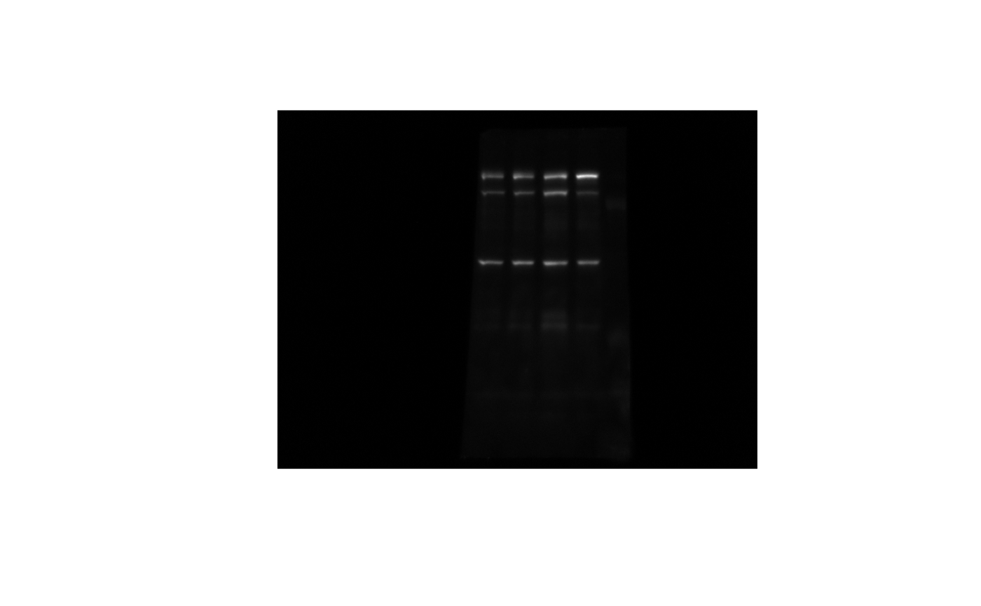

We’re also going to create column and row annotations while we’re at it.

Column annotations are probably the most involved, so we’ll start with them.

To make the column annotation, create a data.frame that has one row per lane in the blot. The columns should represent experimental conditions. The order of the rows should be the order of the columns after image manipulation. This is important, as these images are mirrored - we’ll flip them the right way once we get on to image manipulation.

ca <- data.frame(
  drug = c("DMSO", "Erdafitinib", "Erdafitinib", "Erdafitinib"),
  time_hr = c(0, 24, 48, 72)
)

Row annotation can be supplied as a data.frame with just one column - name - or, much more simply, as a character vector, which is what we’ll do here. The order should match the order of images.

With that, we have everything we need:

wb <- wb(
  imgs = c(parp, trail, actin),
  col_annot = ca,
  row_annot = c("PARP", "TRAIL", "Actin")
)

Editing blots

Now that we have a blot object, we can call wb_visual_edit on it to help us generate code to transform out blots:

wb_visual_edit(wb)

After editing your individual blots and clicking “done”, the app will quit and the code to write the transformations will appear in your console:

Paste in your script to crop the images as seen in the app:
transforms(wb) <- tibble::tribble(
  ~width, ~height, ~xpos, ~ypos, ~rotate, ~flip,
    190L,     60L,   269,    51,    -0.5,  TRUE,
    190L,     50L,   238,   276,       0,  TRUE,
    190L,     30L,   283,   206,       0,  TRUE
  )

Doing so, we get:

transforms(wb) <- tibble::tribble(
  ~width, ~height, ~xpos, ~ypos, ~rotate, ~flip,
    190L,     60L,   269,    51,    -0.5,  TRUE,
    190L,     50L,   238,   276,       0,  TRUE,
    190L,     30L,   283,   206,       0,  TRUE
  )
wb
#> $imgs
#> # A tibble: 3 × 7
#>   format width height colorspace matte filesize density
#>   <chr>  <int>  <int> <chr>      <lgl>    <int> <chr>  
#> 1 TIFF     696    520 Gray       FALSE   728306 83x83  
#> 2 TIFF     696    520 Gray       FALSE   728306 83x83  
#> 3 TIFF     696    520 Gray       FALSE   728306 83x83  
#> 
#> $col_annot
#>          drug time_hr
#> 1        DMSO       0
#> 2 Erdafitinib      24
#> 3 Erdafitinib      48
#> 4 Erdafitinib      72
#> 
#> $row_annot
#>    name
#> 1  PARP
#> 2 TRAIL
#> 3 Actin
#> 
#> $transforms
#> # A tibble: 3 × 6
#>   width height  xpos  ypos rotate flip 
#>   <int>  <int> <dbl> <dbl>  <dbl> <lgl>
#> 1   190     60   269    51   -0.5 TRUE 
#> 2   190     50   238   276    0   TRUE 
#> 3   190     30   283   206    0   TRUE 
#> 
#> attr(,"class")
#> [1] "wb"

Note that the transforms have not been applied: the imgs are still the width and height that they were before updating the transformations. This allows you to re-edit the blots if you so desire. The transformations can manually be applied using apply_transforms, but they are also automatically applied upon present_wb:

wb_present(wb)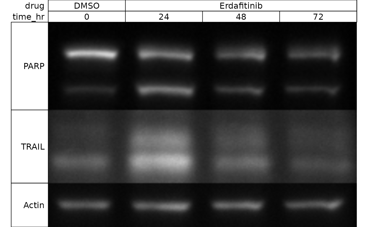

You’ll note that our annotations have automatically been applied - isn’t that nice!

If you want to exclude certain proteins, you can index by row just like a data.frame:

wb_present(wb[-2,])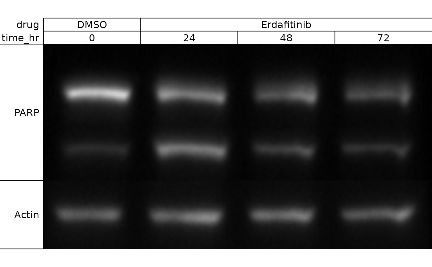

You can additionally select lanes as though they were columns:

wb_present(wb[, 2:4])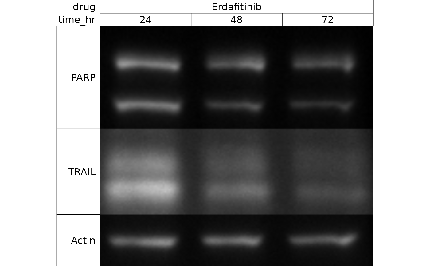

In practice, this will allow you to do some pretty un-recommended things - but by providing the code, at least it’s auditable.

Introduction

Creating a wb object

Editing blots

Creating a `wb` object